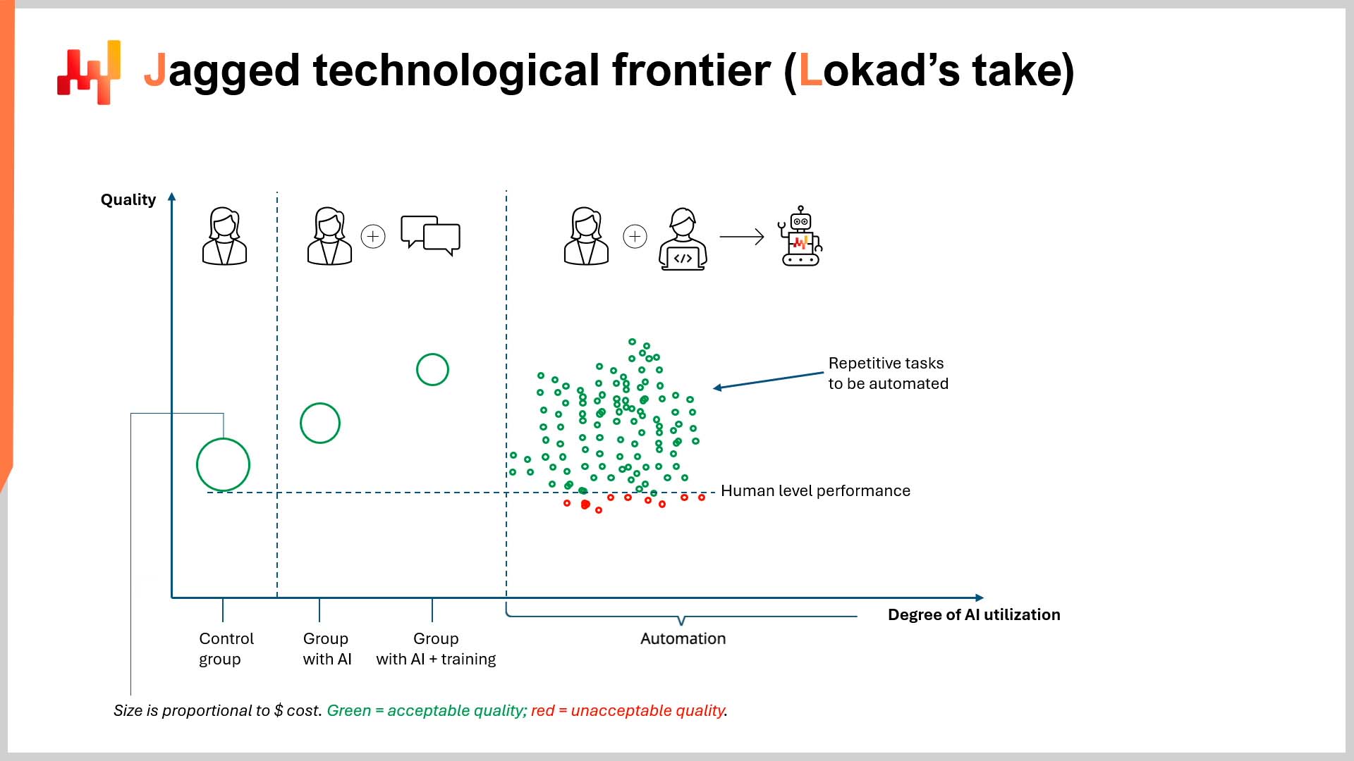
About this blog

Lokad staff posts here tips, news and tutorial either related to Lokad or related to business forecasting in general.

Check our archives for a selection of posts to help your business with insights about forecasting.

Wednesday
May232012

Whitepaper on Out-of-Shelf Monitoring Technology released

Few aspects of retailing are as fundamental as fully stacked shelves, and few concerns rank higher with an ever more demanding customer than product availability. Regardless, on-shelf availability remains a huge challenge for the industry. Growing, more dynamic product portfolios, staff and cost cuts combined with an increasingly complex supply chain have increased the challenge.

Cover of the OOS whitepaper by LokadWhile shelf availability is a top concern for customers and retailers alike, even the Tier I retailers today mostly rely on manual checks by store staff. This puts a large burden on employees, and response times to out-of-shelf situations are slow.

However, grocery retailers a crossed Europe and the US have started to explore technology that can help address the problem. With this in mind, we have published a whitepaper on out-of-shelf monitoring technology which gives an overview of

  • Objectives of out-of-shelf monitoring systems
  • Introduction to the technology
  • Definition of performance characteristics
  • Quantification of system capabilities and limitations

Are we missing some interesting aspects of this type of technology, or do you have experience with OOS monitoring systems you want to share? Please let us know in the comments.

Wednesday
May162012

ROI = Return On Inventory?

ROI stands of course for return on investment. However, the idea that every euro or dollar ‘invested’ in inventory brings a certain return in terms of profits is a powerful thought. When looking at inventory from this angle, two questions arise:

  • Are profits earned by a product versus the capital invested in stocking it (i.e. ROI) similar over the product portfolio?
  • If the ROIs of the various products are heterogeneous – how can the overal ROI delivered by the inventory be maximized?

ROI meter As you will have guessed, the answer to the first question is a clear ‘NO’. The return generated by a product for the euros invested in stocking it differs vastly from product to product. Two aspects have a major impact.

First, the gross margin of a product directly affects the ROI. This is obvious, and product managers naturally try to build a portfolio with high margins in mind. However, many other considerations come into play such as the coverage of the product portfolio for example. Adding more products to the portfolio is often also a strategy for growth.

The second aspect is more subtle, but equally important: The amount of stock that is required to provide a desired availability (i.e. service level) varies significantly among products. The main driver here is the volatility of demand - the higher the uncertainty of the future demand, the higher the inventory level required to assure a given service level.

As an example, lets imagine two products with the same gross margin that sell the same number of units during the year, thus generating the same amount of annual gross profit. However, product A sells the same amount each week with a high certainty, while product B is much more erratic with no sales for weeks and large orders in others. To achieve the same availability or service level for both products, the safety stock for product B will be a lot higher than for product A, where very little uncertainty and therefore safety stock requirement is given. As a result, product B requires much more units in stock than product A to achieve the same annual profit. The ROI for product A is therefore significantly higher.

Inventory is moneyBusinesses continually work on maximizing their return on capital employed (ROCE). Inventory is a significant part of the capital invested by most retailers, and therefore an important opportunity for optimization. The good news is that the potential for optimizing the ROI of your inventory by taking advantage of the heterogeneous ROIs across your catalog is large.

The latter is done by finding the optimal service level at which an SKU produces the best ROI within the constraint of a set inventory budget. As a result availability and revenue can be increased for a given inventory budget, or cash can be released from inventory while maintain the overall availability.

The analysis behind this optimization however is not trivial given the non-linear correlation between service level and inventory levels. Additionally, a set of ‘strategic’ constraints such availability goals for certain products need to be taken into account. 

This is a challenge which we plan to take on in the near future, the goal being a fully automated ROI optimization over the product portfolio for a given working capital sum. As an output, the system will determine service levels per SKU that give the highest availability (and therefore revenues) for a chosen inventory budget.

Excessive inventory reduces the return on invested capital, but too little inventory diminishes profits as well. The optimal inventory level is therefore a trade-off between stock-out cost and inventory cost, and falling too far on either side of the optimum will negatively impact your business. Our plans for service level optimization will leverage our forecasting technology. Stay tuned.

Tuesday
May082012

Sparsity: when accuracy measure goes wrong

Three years ago, we were publishing Overfitting: when accuracy measure goes wrong, however overfitting is far from being the only situation where simple accuracy measurements can be very misleading. Today, we focus on a very error-prone situation: intermittent demand which is typically encountered when looking at sales at the store level (or Ecommerce).

We believe that this single problem alone has prevented most retailers to move toward advance forecasting systems at the store level. As with most forecasting problems, it's subtle, it's counterintuitive, and some companies charge a lot to bring poor answers to the question.

Illustration of intermittent sales

The most popular error metrics in sales forecasting are the Mean Absolute Error (MAE) and the Mean Absolute Percentage Error (MAPE). As a general guideline, we suggest to stick with the MAE as the MAPE behaves very poorly whenever time-series are not smooth, that is, all the time, as far retailers are concerned. However, there are situations where MAE too behaves poorly. Low sales volumes fall in those situations.

Let's review the illustration here above. We have an item sold over 3 days. The number of unit sold over the first two days is zero. On the third day, one unit get sold. Let's assume that the demand is, in fact, of exactly 1 unit every 3 days. Technically speaking, it's a Poisson distribution with λ=1/3.

In the following, we compare two forecasting models:

  • a flat model M at 1/3 every day (the mean).
  • a flat model Z at zero every day.

As far inventory optmization is concerned, the model zero (Z) is downright harmfull. Assuming that safety stock analysis will be used to compute a reorder point, a zero forecast is very likely to produce a reorder point at zero too, causing frequent stockouts. An accuracy metric that would favor the model zero over more reasonable forecasts would be behaving rather poorly.

Let's review our two models against the MAPE (*) and the MAE.

  • M has a MAPE of 44%.
  • Z has a MAPE of 33%.
  • M has a MAE of 0.44.
  • Z has a MAE of 0.33.

(*) The classic definition of MAPE involves a division by zero when the actual value is zero. We assume here that the actual value is replaced by 1 when at zero. Alternatively, we could also have divided by the forecast (instead of the actual value), or use the sMAPE. Those changes make no difference: the conclusion of the discussion remains the same.

In conclusion, here, according to both the MAPE and the MAE, model zero prevails.

However, one might argue that this is simplistic situation, and it does not reflect the complexity of a real store. This is not entirely true. We have performed benchmarks over dozens of retail stores, and usually the winning model (according to MAE or MAPE) is the model zero - the model that returns always zero. Futhermore, this model typically wins by a comfortable margin over all the other models.

In practice, at store level, relying either on MAE or MAPE to evaluate the quality of forecasting models is asking for trouble: the metric favors models that return zeroes; the more zeroes, the better. This conclusion holds for about every single store we have analyzed so far (minus the few high volume items that do not suffer this problem).

Readers who are familar with accuracy metrics might propose to go instead for the Mean Square Error (MSE) which will not favor the model zero. This is true, however, MSE when applied to erratic data - and sales are store level are erratic - is not numerically stable. In practice, any outlier in the sales history will vastly skew the final results. This sort of problem is THE reason why statisticians have been working so hard on Robust statistics in the first place. No free lunch here.

How to assess store level forecasts then?

It took us a long, long time, to figure out a satifying solution to the problem of quantifying the accuracy of the forecasts at the store level. Back in 2011 and before, we were essentially cheating. Instead of looking at daily data points, when the sales data was too sparse, we were typically switching to weekly aggregates (or even to monthly aggregates for extremely sparse data). By switching to longer aggregation periods, we were artificially increasing sales volumes per period, hence making the MAE usable again.

The breakthrough came only a few months ago through quantiles. In essence, the enlightenment was: forget the forecasts, only reorder points matter. By trying to optimize our classic forecasts against metrics X, Y or Z, we were trying to solve the wrong problem.

Wait! Since reorder points are computed based on the forecasts, how could you say forecasts are irrelevant?

We are not saying that forecasts and forecast accuracy are irrelevant. However, we are stating that only the accuracy of the reorder points themselves matter. The forecast, or whatever other variable is used to compute reorder points, cannot be evaluated on its own. Only accuracy of the reorder points need and should be evaluated.

It turns out that a metric to assess reorder points exists: it's the pinball loss function, a function that has been known by statisticians for decades. Pinball loss is vastly superior not because of its mathematical properties, but simply because it fits the inventory tradeoff: too much stocks vs too much stockouts.

Wednesday
May022012

Video: Quantile Forecasts - Part 2

Last week, we published the Quantile Forecasts - Part 1 video; here comes the Part 2. In the previous video, we discussed what quantiles were about. In short, it's a new way to look at the inventory optimization mechanism itself.

In Part 2, we provide some non-technical insights why quantile forecasts outperforms classic ones in three usual situations.

Video summary (7min46):

  • High service levels
  • Intermittent demand
  • Spiky demand

Don't hesitate to post questions in comments.

Wednesday
Apr252012

Video: Quantile Forecasts - Part 1

Quantile forecasts offer a radically new and better way to compute optimal reorder points. Here is our first video about this little supply chain breakthrough.

Video summary (6min25):

  • What are quantiles?
  • How do quantiles work?
  • What are the advantages of quantiles?

Stay tuned for more.

Saturday
Apr142012

Out-of-shelf trilemma

Shopping Cart logo Most people are familiar with the notion of dilemma when two possibilities are offered neither of which being acceptable. Safety stock analysis is a classical mathematical dilemma: you can choose between more stocks or more stockouts, yet both of them generate extra costs.

However, it exists situations where the trade-off is more complex in the sense there are more than 2 unfavorable options to balance. When there are 3 unfavorable options to be balanced, the situation is called a trilemma.

Out-of-shelf (OOS) monitoring, ala Shelfcheck, is facing a trilemma when it comes to the quality of the alerts being delivered:

  • Sensibility, the percentage of OOS problems being captured.
  • Precision, the percentage of true alerts within all OOS alerts.
  • Latency, the delay between then start of the OOS problem and the alert.

Pick any two, but you can't have them all. In fact, for any given demand forecasting accuracy, improving any of those 3 metrics come at the expense of the 2 other metrics.

Monday
Mar122012

Quantiles = Inventory Optimization 2.0

Quantile Logo Getting more accurate forecasts, that turn into profits, is the No1 priority for Lokad. However, demand forecasting has been extensively researched for more than a half a century, and each 0.1% of extra accuracy is typically nothing less than a uphill battle.

Sometimes though, we make a breakthrough. Today, we are announcing the most significant technology upgrade of Lokad since its launch 6 years ago: the immediate availability of quantile forecasts.

Quantiles are disruptive in the sense that in many situations they make classic forecasts plain obsolete as far inventory optimization is concerned - for retail, wholesale and manufacturing businesses.

We have identified 3 situations where quantiles really shine:

  • High service levels at 90% and above.
  • Intermittent demand (slow mover's).
  • Bulk orders (spiky demand).

In those situations, benchmarks against our own classic forecasting technology indicate that quantile forecasts typically bring either 20% less inventory or 20% less stockouts.

Extraordinary claims require extraordinary evidence. Carl Sagan

However, the many benchmarks that we have made so far with our prospects and clients indicate that our classic forecasting technology is already ahead of the competition; but with quantile forecasts, it's whole new level of inventory optimization that can be achieved.

Don't hesitate to put quantiles to the test.

The story behind the quantile upgrade

Quantile forecasting (also called quantile regression) has been around for decades among academic circles. Then, in finance, analysts have been extensively using quantiles for Value at Risk (VaR) analysis since the late 1980s.

At Lokad, quantiles have been around for a long time as well. For example, back in 2009, Sequential Quantile Prediction of Time Series. IEEE Transactions on Information Theory, March 2011, vol. 57, n°3 has been published by one of us. However, until very recently, quantiles were very mistakenly considered a mathematical distraction (business-wise) rather than a mission critical concept.

What did hold us back was not lacking insights in statistics, but lacking insights in the profound relationship between quantiles and inventory optimization. This insight was triggered, mostly out of dumb luck, when a client did ask us to figure out a formula to compute optimal service levels for her inventory.

A breakthrough yes, but a late one

This quantile breakthrough is only very relative in the sense that quantiles have been already applied successfully for decades in other trades. However, there is one aspect that partially explains this late arrival: quantile models typically require about 10x more processing power compared to classic forecasting models. Without cloud computing, we would not have been able to put quantiles in production, while preserving an aggressive pricing.

Monday
Feb202012

How much do you get for 1% extra accuracy?

One of the problems that comes with being specialists of a subject is that you tend to take for granted what is obscure for anyone but your peers. At Lokad, despite our best efforts, we are no exception, especially when it comes to forecasting...

Recently, we realized that we had never provided any in-depth quantitative assessment of the financial gains generated by an increase of the forecasting accuracy, which is about the raison d'être for the company. Furthermore, after investigating the web, we realized that other forecasting vendors (competitors) were rather fuzzy too about the financial rewards that could be achieved through better forecasts.

However, it's not that complicated. With the following variables:

  • $D$ the turnover (total annual sales).
  • $m$ the gross margin.
  • $\alpha$ the cost of stockout to gross margin ratio.
  • $p$ the service level achieved with the current error level (and current stock level).
  • $\sigma$ the forecast error of the system in place, expressed in MAPE (mean absolute percentage error).
  • $\sigma_n$ the forecast error of the new system being benchmarked (hopefully lower than $\sigma$).

The yearly benefit $B$ of going for the new forecasting system is given by:

$$B = D (1 - p) m \alpha \frac{\sigma - \sigma_n}{\sigma}$$

For the proof of this result, check the full length article.

Wednesday
Jan252012

Optimal service level and order quantity

In the inventory optimization literature, one of the most recurring concepts is the service level, i.e. the desired probability of not hitting a stock-out situation. The service level expresses the tradeoff between too much inventory and too many stock-outsHowever, experts remain typically vague when it comes to choose service level values; a pattern also followed by most inventory software products...

That's why we have spent a bit of time to craft a formula that gives optimal service levels. Naturally, the optimality is not obtained without assumptions. However, we believe those are reasonable enough to preserve the efficiency of the formula for most businesses.

Then, another subject, that receives too little attention, is the optimal order quantity: the quantity to be ordered in order to minimize the combination of purchase costs, carrying costs, shipping costs, etc. As of January 2012, it's fascinating to notice that most of the industry still relies on the Wilson formula devised back in 1913. Yet, this formula comes with strong assumptions that do not make much sense any more for the supply chain of the 21st century.

Thus, we have designed another economic order quantity formula that emphasizes volume discounts (instead of a flat ordering cost) for larger purchases. The formula (or rather the approach) is fairly general, and could be applied to any pricing structure, including non-linear situations where specific quantities are favored because they matche the size of a crate or a pallet.

Both situations are illustrated with Excel sheets (so you don't even need Lokad to get started).

Tuesday
Jan032012

Big data in retail, a reality check

Cloud computing being so 2011, big data is going to be a key IT buzzword for 2012. Yet, as far we understand our retail clients, there is one data source that holds above 90% of total information value in their possession: market basket data (tagged with fidelity card information when available).

For any mid-large retail network, the informational value of market basket data simply dwarfs about all other alternative data sources, may it be:

  • In-store video data, which remain difficult to process, and primarily focused on security.
  • Social media data, which are very noisy and reflect as much bot implementations than human behaviors.
  • Market analyst’s reports, which require the scarcest resource of all: management attention.

Yet, beside basic sales projections (aka sales per product, per store, per region, per week …), we observe that, as of January 2012, most retailers are doing very little out of their market basket data. Even forecasting for inventory optimization is typically nothing more than a moving average variant at the store level. More elaborate methods are used fore warehouses, but then, retailers are not leveraging basket data anymore, but past warehouse shipments.

Big Data vendors promise to bring an unprecedented level of data processing power to their clients to let them harness all the potential of their big data. Yet, is this going to bring profitable changes to retailers? Not necessarily so.

The storage capacity sitting on display on the shelves of an average hypermarket with +20 external drives in display (assuming 500GB per drive) typically exceeds the raw storage needed to persist a whole 3 years of history of a 1000 stores network (i.e. 10TB of market basket data). Hence, raw data storage is not a problem, or, at least, not an expensive problem. Then, data I/O (input/output) is a more challenging matter, but again, by choosing an adequate data representation (the details would go beyond the scope of this post), it’s hardly a challenge as of 2012.

We observe that the biggest challenge posed by Big Data is simply manpower requirements to do anything operational with it. Indeed, the data is primarily big in the sense that the company resources, to run the Big Data software and to implement whatever suggestions come out of it, are thin.

Producing a wall of metrics out of market basket data is easy; but it’s is much harder to build a set of metrics worth the time being read considering the hourly costs of employees.

As far we understand our retail clients, the manpower constraint alone explains why so little is being been done with market basket data on an ongoing basis: while CPU has never been to cheap, staffing has never been so expensive.

Thus, we believe that Big Data successes in retail will be encountered by lean solutions that treat, not processing power, but people, as the scarcest resource of all.